Abstract

The project obtains Ontario Gas Demand from tsdl library and analyzed it with linear time series models and I fitted the data with SARIMA(3,0,3)(4,1,2) ₁₂ which corrected predicted the gasoline demand of next cycle after various transformation and differencing.

1.Introduction

Given current high inflation environment and sky-rocketing gasoline price, it is of the interest to analysis how demand of Gasoline changes over time. There is a data collected in TSDL library of gasoline demand in Ontario province.

2.Data modeling

2.1 Data collection

  
library(tsdl)
options(warn=-1)
tsdl_gasdemand <- subset(tsdl, "Sales")
X_t <- tsdl_gasdemand[[1]]
attributes(X_t)

$tsp
[1] 1960.000 1975.917   12.000

$class
[1] "ts"

$source
[1] "Abraham & Ledolter (1983)"

$description
[1] "Monthly gasoline demand Ontario gallon millions 1960 – 1975"

$subject
[1] "Sales"

2.2 Data spilting

Total of 192 observations, make 12 obs as test data set and rest as train data set

  
train <- X_t[1:180]
test <- X_t[181:length(X_t)]
plot.ts(train, main="Monthly gasoline demand Ontario 1960 – 1975 training data") 
fit <- lm(train ~ as.numeric(1:length(train)))
abline(fit, col="red")
abline(h=mean(train), col="blue")

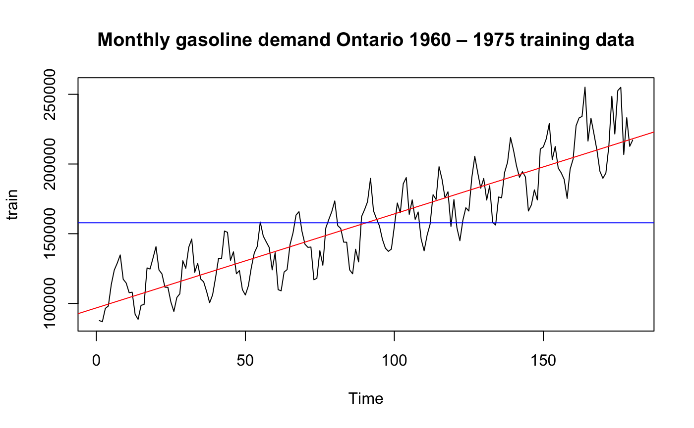
Clearly this data has trend and it is symmetric so it may fit a linear model we have learned

2.3 Normality Check of Training data

  
par(mfrow=c(1,2))
hist(train, col="mediumorchid1", xlab="", 
     main="Histogram of X_t",freq = F,density = 20) 
m <- mean(train)
std <- sqrt(var(train))
curve(dnorm(x, m, std), col="red", add=TRUE,yaxt = "n")
qqnorm(train)
qqline(train,col="indianred2")

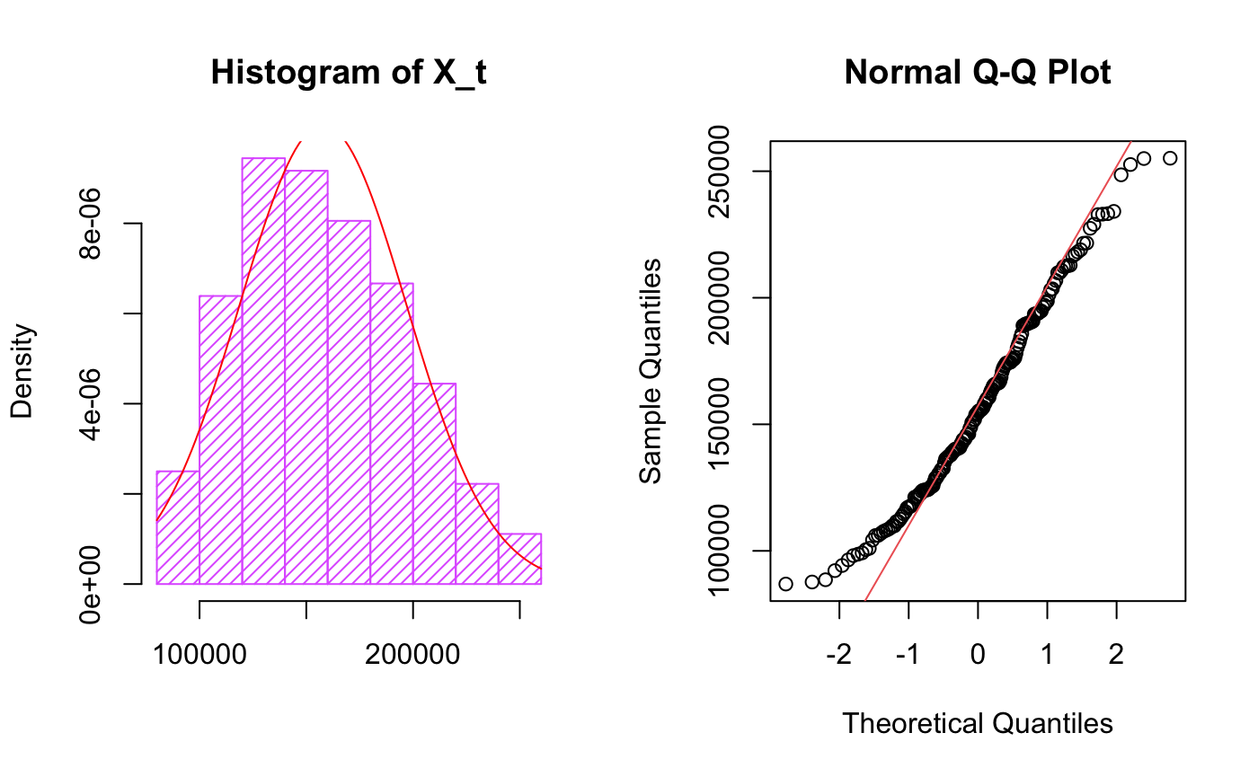
It follows normal distribution with some skew by looking at histogram plots, QQ plot suggests there are outliers.

2.4 ACF/PACF of Training data

  
par(mfrow=c(1,2))
acf(train, lag.max=50, main="ACF of training set")
pacf(train, lag.max=50, main="PACF of training set")

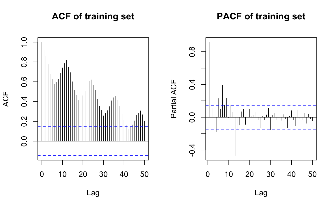
it looks like differencing is needed as there is seasonality(monthly) in ACF and strong peak at lag12 in PACF

2.5 Decomposition and transformation of train data

  
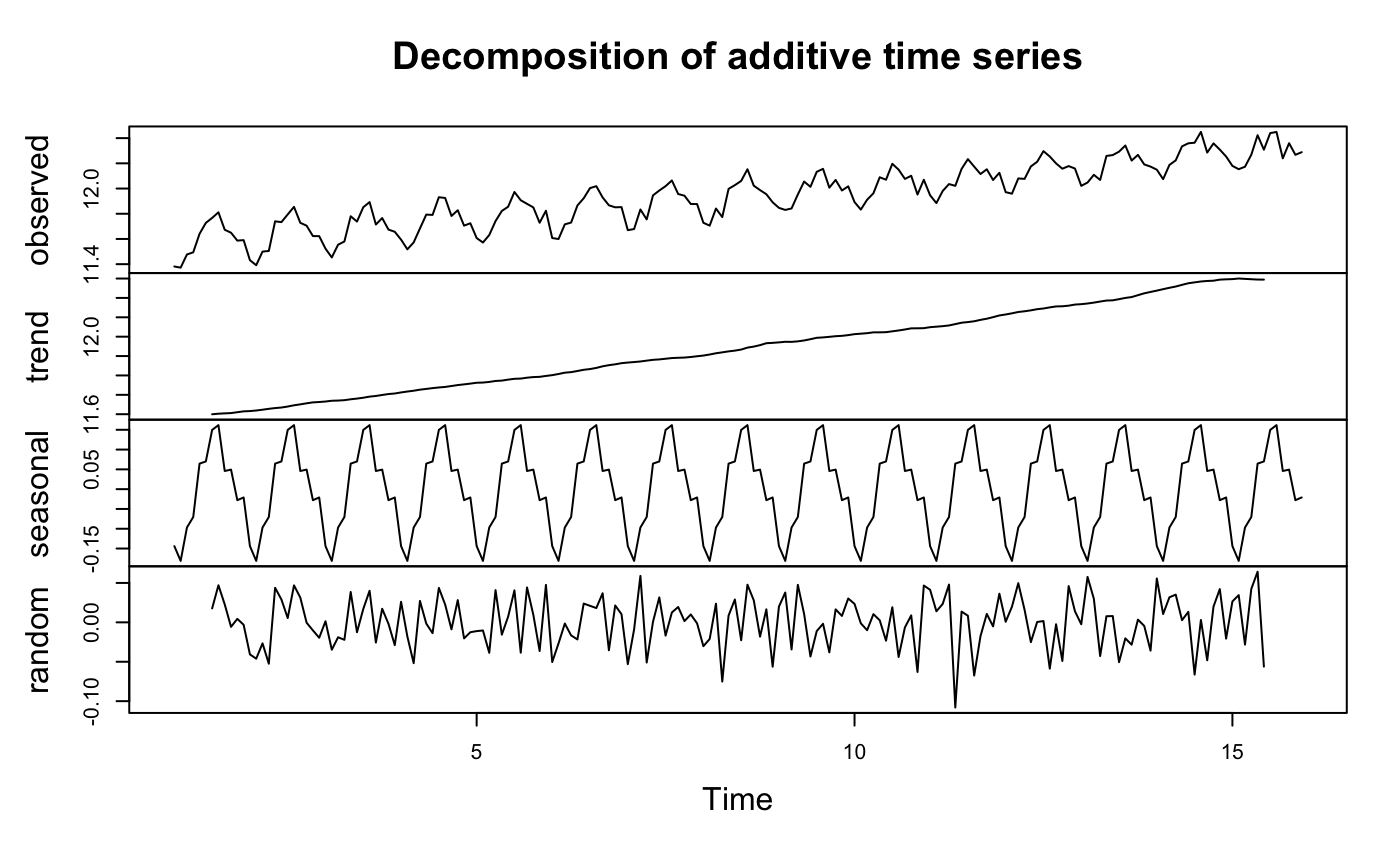
y <- ts(as.ts(train), frequency = 12) 
decomp <- decompose(y)
plot(decomp)

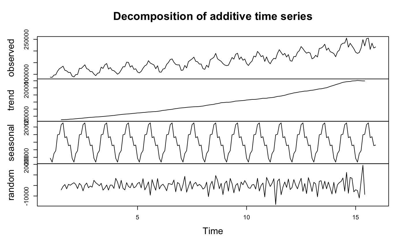
we can see there is seasonal component and trend which confirms previous conclusion again. To remove trend, transform data or take difference.

\begin{eqnarray} f_\lambda\left(U_t\right)= \begin{cases}\lambda^{-1}\left(U_t^\lambda-1\right), & U_t\geq 0, \lambda>0 \\ \ln U_t, & U_t>0, \lambda=0\end{cases} \notag \end{eqnarray}

  
library(MASS)
t = 1:length(train)
fit = lm(train ~ t)
bcTransform = boxcox(train ~ t,plotit = TRUE)
lambda = bcTransform$x[which.max(bcTransform$y)] 
train.log= log(train)

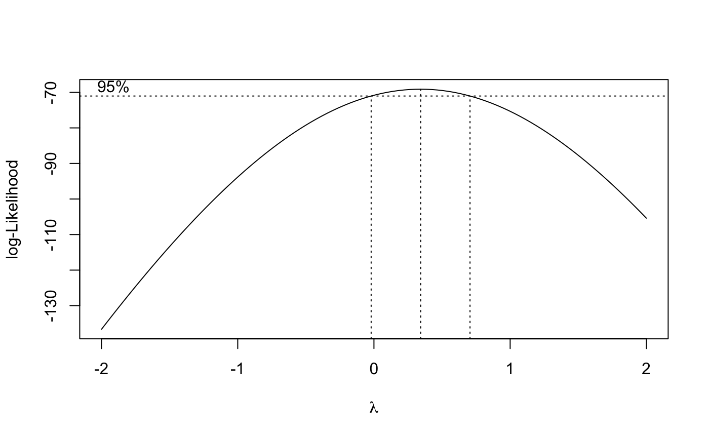
because box-cox test suggest log transformation($\lambda \geq 0$), I will adopt log transformation method first.

  
par(mfrow=c(2,2))
plot.ts(train.log,main = "log transformed data")
plot.ts(train,main = "Original data")
hist(train.log, col="slateblue4", 
     main="Histogram of the log Transformed Data",
     freq = F,
     density = 20)
m1 <- mean(train.log)
std1 <- sqrt(var(train.log))
curve(dnorm(x, m1, std1), col="firebrick1", add=TRUE)
qqnorm(train.log, main="Normal Q-Q Plot of train.log")
qqline(train.log,col ="blue")

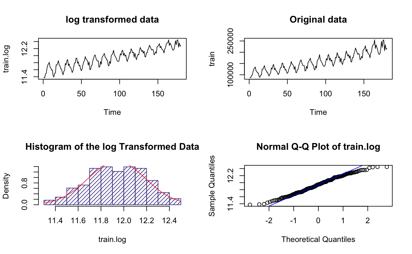
The range(y-axis) became much smaller but others look like the same, suggesting higher variance

It’s roughly normal based on the histogram plot

  
y.log <- ts(as.ts(train.log), frequency = 12) 
decomp.log <- decompose(y.log)
plot(decomp.log)

It is clear we need to do difference because there is trend even after log transformation

3 Data transformation

3.1 Difference time series(log transformed)

  
suppressMessages(library(forecast))
diffs <- diff(train.log,12) #remove seasonality
ddiffs <- diff(diffs,1)# remove trend

ts_var <- c(var(train.log),var(diffs),var(ddiffs))
ts_var_descrb <- c("Var of log TS","Var of  diffs",
                   "Var of ddiffs")
df <- data.frame(ts_var_descrb,ts_var)
df
ts.plot(diffs, main="De-seasonlized Time Series",
        ylab=expression(nabla[12]~Y[t]))
abline(h=mean(diffs), lty=2)
fitdiff <- lm(diffs ~ as.numeric(1:length(diffs)))
abline(fitdiff, col="red")

ts_var_descrb
<chr>  ts_var   <dbl>
Var of log TS	0.062973684			
Var of diffs	0.001643779			
Var of ddiffs	0.003746485

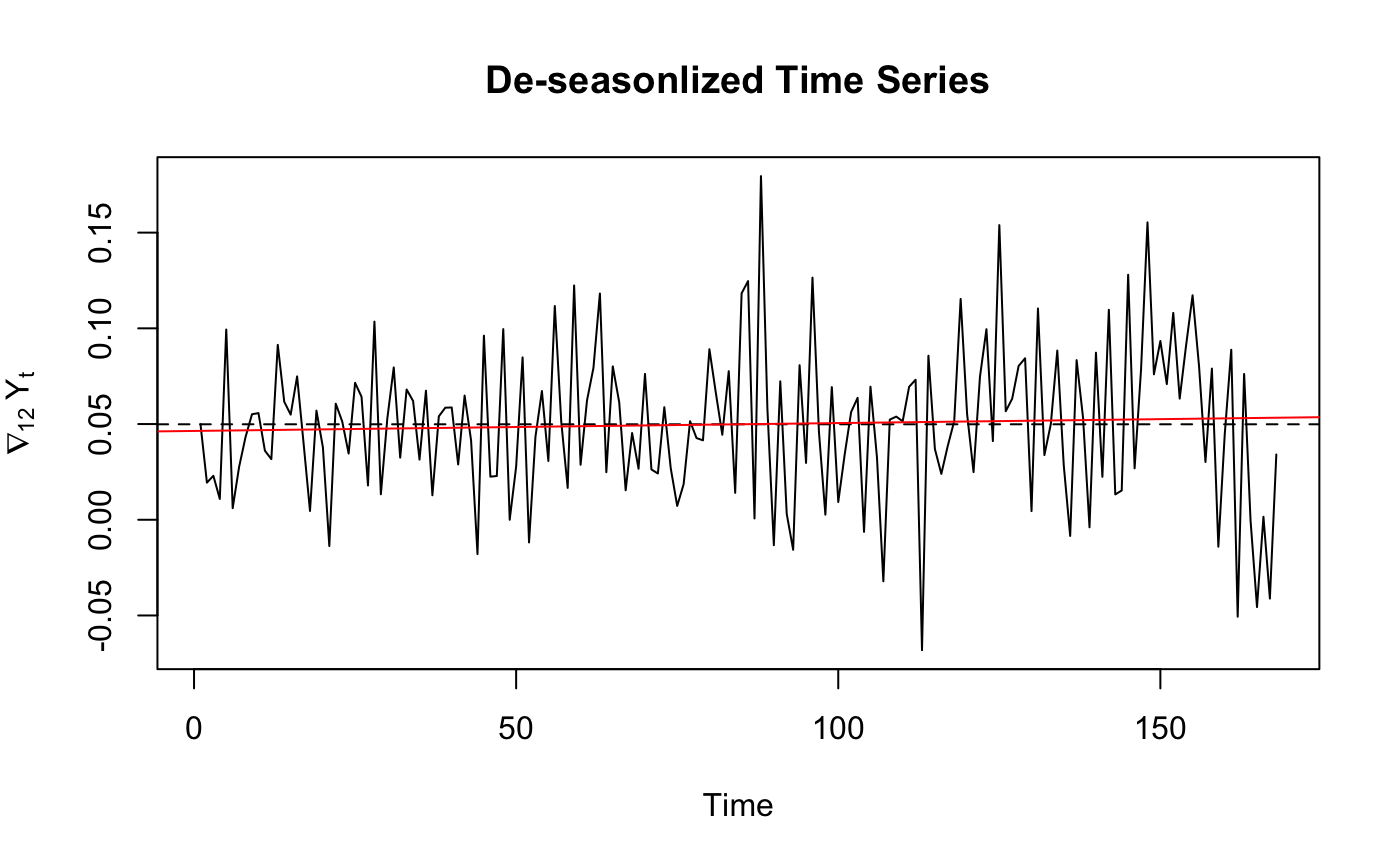
From the variance comparison list we can see that for log transformed Time Series , difference once at lag 12 have lowest variance.So we chose to use diffs to plot ACF/PACF.

3.2 Histagram of De-seasonal data

  
par(mfrow=c(1,2))
hist(diffs, col="light blue", xlab=expression(nabla[12]~(X[t]^{ln})), prob=TRUE,density = 40) 
m <- mean(diffs)
std <- sqrt(var(diffs)) 
curve(dnorm(x,m,std), add=TRUE,col="red")
qqnorm(diffs, main="Normal Q-Q Plot of diffs")
qqline(diffs,col ="blue")

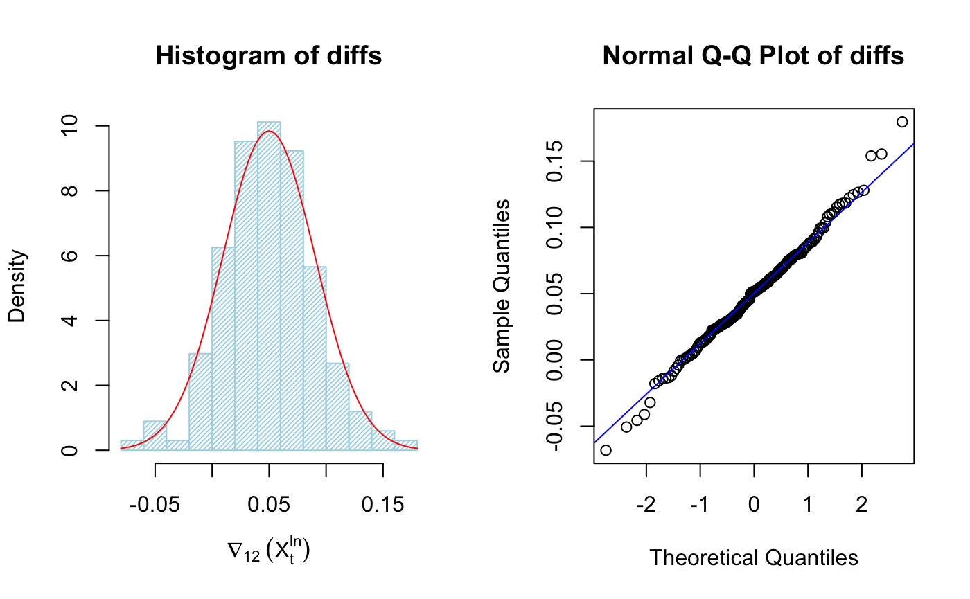
It’s clear the data is much more “Gaussian”, we can plot ACF/PACF of differenced transformed data

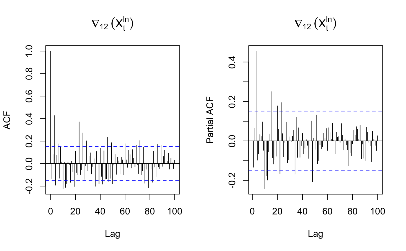
3.3 ACF/PACF of differenced trainging data

  
par(mfrow=c(1,2))
acf(diffs, lag.max=100, main=expression(nabla[12]~(X[t]^{ln})))
pacf(diffs, lag.max=100, main=expression(nabla[12]~(X[t]^{ln})))

3.4 Model parameter identification

seasonal part
D=1 – Differenced once at lag 12
s= 12 – 12 month per year
P=4 – strong peak at multiple of lag 12 before lag 60 in PACF
Q could be 1,2,3,4 based on the multiple of ACF.

non-seasonal part
p = 3 – strong peak at lag 3
d = 0 – not differenced at lag 1
q = 3 – strong peak at lag 3 in ACF

That gives SARIMA(3,0,3)x(4,1,c(1,2,3,4))₁₂

4.0 Model fitting

  
suppressMessages(library(astsa))

model1 <- sarima(xdata=train.log, p=3, d=0, q=3, P=4, D=1, Q=1, S=12, details = F)
model2 <- sarima(xdata=train.log, p=3, d=0, q=3, P=4, D=1, Q=2, S=12, details = F)
model3 <- sarima(xdata=train.log, p=3, d=0, q=3, P=4, D=1, Q=3, S=12, details = F)
model4 <- sarima(xdata=train.log, p=3, d=0, q=3, P=4, D=1, Q=4, S=12, details = F)

4.1 AICC check

  
AICc_value <- c(model1$AICc,model2$AICc,model3$AICc,model4$AICc)
AICc_des <- c("AICC of Model1","AICC of Model2","AICC of Model3","AICC of Model4")
df_AICC <- data.frame(AICc_des,AICc_value)
df_AICC

AICc_des        AICc_value
<chr>           <dbl>
AICC of Model1	-4.076983			
AICC of Model2	-4.135593			
AICC of Model3	-4.133020			
AICC of Model4	-4.129460	

Based on AICC value, we can chose model 2 which is SARIMA(3,0,3)(4,1,2)$_{12}$

  
model2$fit
model2$AICc

Call:
arima(x = xdata, order = c(p, d, q), seasonal = list(order = c(P, D, Q), period = S), 
    xreg = constant, transform.pars = trans, fixed = fixed, optim.control = list(trace = trc, 
        REPORT = 1, reltol = tol))

Coefficients:
          ar1      ar2     ar3     ma1     ma2     ma3    sar1     sar2     sar3     sar4     sma1
      -0.2531  -0.1308  0.2677  0.2831  0.3681  0.2317  0.1603  -0.6132  -0.4573  -0.3213  -0.9767
s.e.   0.1585   0.1437  0.1620  0.1655  0.1380  0.1685  0.2127   0.0834   0.0829   0.1392   0.4181
        sma2  constant
      0.9043    0.0043
s.e.  0.5322    0.0001

sigma^2 estimated as 0.0005733:  log likelihood = 362.57,  aic = -697.14
[1] -4.135593

We need to modify the model because some Coefficient have 0 in their confidence interval.

  
model2_modi <- sarima(xdata=train.log, p=3, d=0, q=3, P=4, D=1, Q=2, S=12, 
                      fixed = c(0,0,0,0,NA,NA,NA,NA,NA,NA,0,0,NA), details = F)
model2_modi$fit
model2_modi$AICc

Call:
arima(x = xdata, order = c(p, d, q), seasonal = list(order = c(P, D, Q), period = S), 
    xreg = constant, transform.pars = trans, fixed = fixed, optim.control = list(trace = trc, 
        REPORT = 1, reltol = tol))

Coefficients:
      ar1  ar2  ar3  ma1     ma2     ma3     sar1     sar2     sar3     sar4  sma1  sma2  constant
        0    0    0    0  0.2555  0.4669  -0.5696  -0.4210  -0.5124  -0.5000     0     0    0.0042
s.e.    0    0    0    0  0.0752  0.0664   0.0711   0.0796   0.0743   0.0734     0     0    0.0001

sigma^2 estimated as 0.0007702:  log likelihood = 353.68,  aic = -691.36
[1] -4.111059

AR1, AR2, AR3, MA1, SMA1, SMA2 term all have 0 in their CI so I have modified them to 0.
The AICC of modified model is higher than original model so we need to use the original model 2 because the coefficients are significant if the AICC of the original model is lower.

4.2 Final Model

so the model selection is

\begin{equation} SARIMA(3,0,3)(4,1,2)_{12} \notag \end{equation}

\begin{equation} (1+0.2531B^1+0.1308B^2-0.2677B^3)(1-0.1603B^{12}+0.6132B^{24}+0.4573B^{36}+0.3213B^{48})X_t=\ \notag \end{equation}

\begin{equation} (1+0.2831B+0.3681B^2+0.2317B^3)(1-0.9767B^{12}+0.9043B^{24})Z_t \notag \end{equation}

5.0 Diagnostic Checking

5.1 Unit Root

  
library(UnitCircle)
par(mfrow=c(2,2))
uc.check(pol_ = c(1,0.2831,0.3681,0.2317), plot_output = TRUE,print_output = F) # Non-Seasonal MA Part
uc.check(pol_ = c(1,0.2531,0.1308,0.2677), plot_output = TRUE,print_output = F)# non-seasonal AR part
uc.check(pol_ = c(1,-0.1603,0.6132,0.4573,0.3213), plot_output = TRUE,print_output = F)# seasonal AR part
uc.check(pol_ = c(1,-0.9767,0.9043), plot_output = TRUE,print_output = F)# seasonal MA part

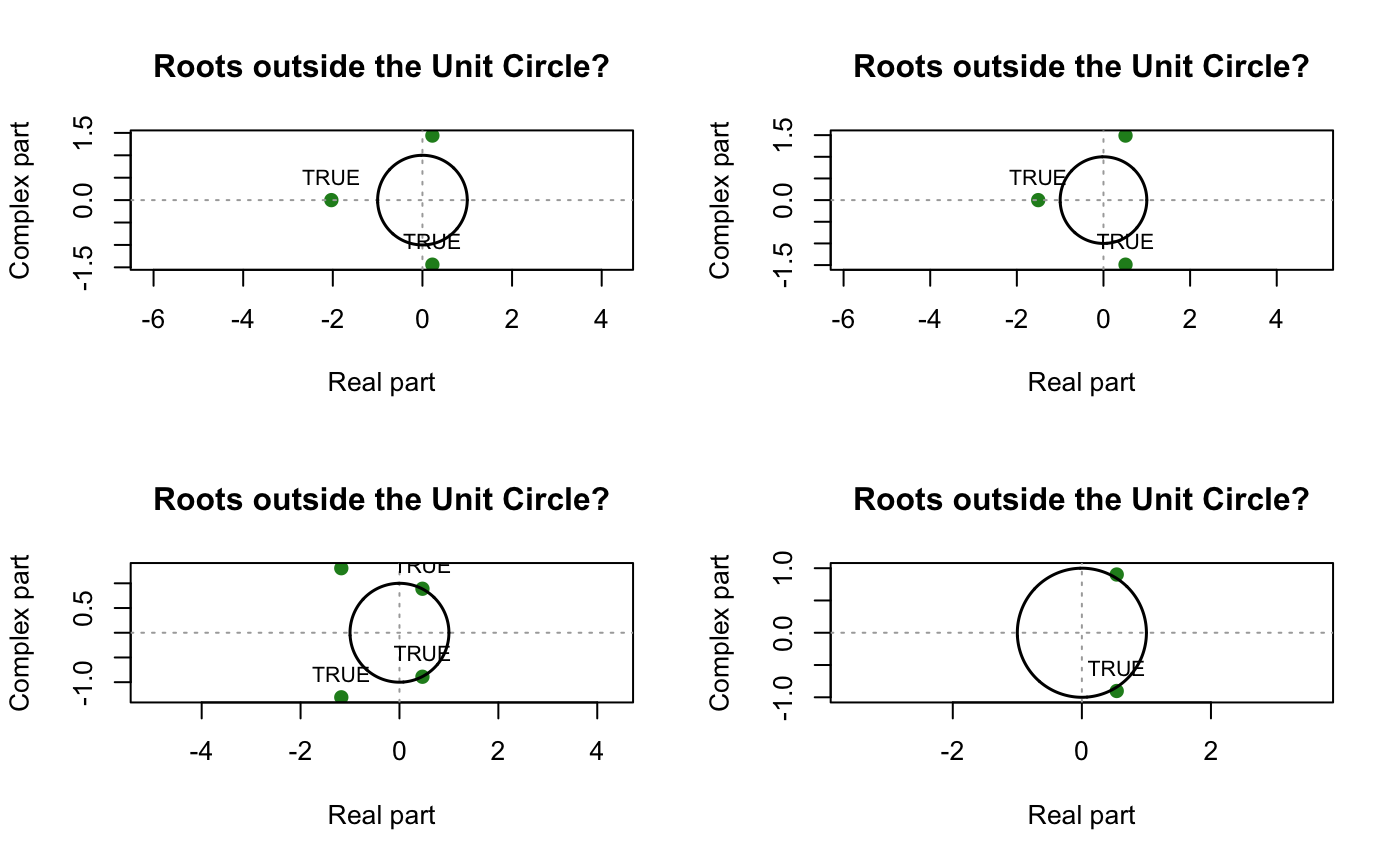
Neither parts has unit root, we proceed to Sanity checking

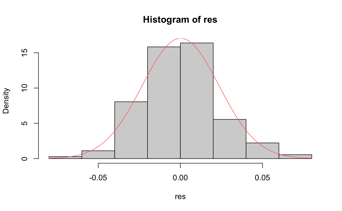
5.2 Residual Normality checking

  
res <- residuals(model2$fit)
res <- tsclean(res)
hist(res,freq = F)
m_res <- mean(res)
std_res <- sqrt(var(res)) 
curve(dnorm(x,m_res,std_res), add=TRUE,col="indianred1")
shapiro.test(res)

    Shapiro-Wilk normality test
data:  res
W = 0.98834, p-value = 0.1452

Shapiro-Wilk normality test

\begin{eqnarray} \begin{cases} H_0: \text{Residuals are normally distributed} \\H_1: \text{not } H_0\end{cases} \end{eqnarray}

it looks like our residuals are normally distributed based on P-value of Shaprio test (>0.05)

  
ts.plot(res, main = "Fitted Residuals") 
abline(h=mean(res), col = "red")
fitres <- lm(res ~ as.numeric(1:length(res)))
abline(fitres, col="blue", lty=2)

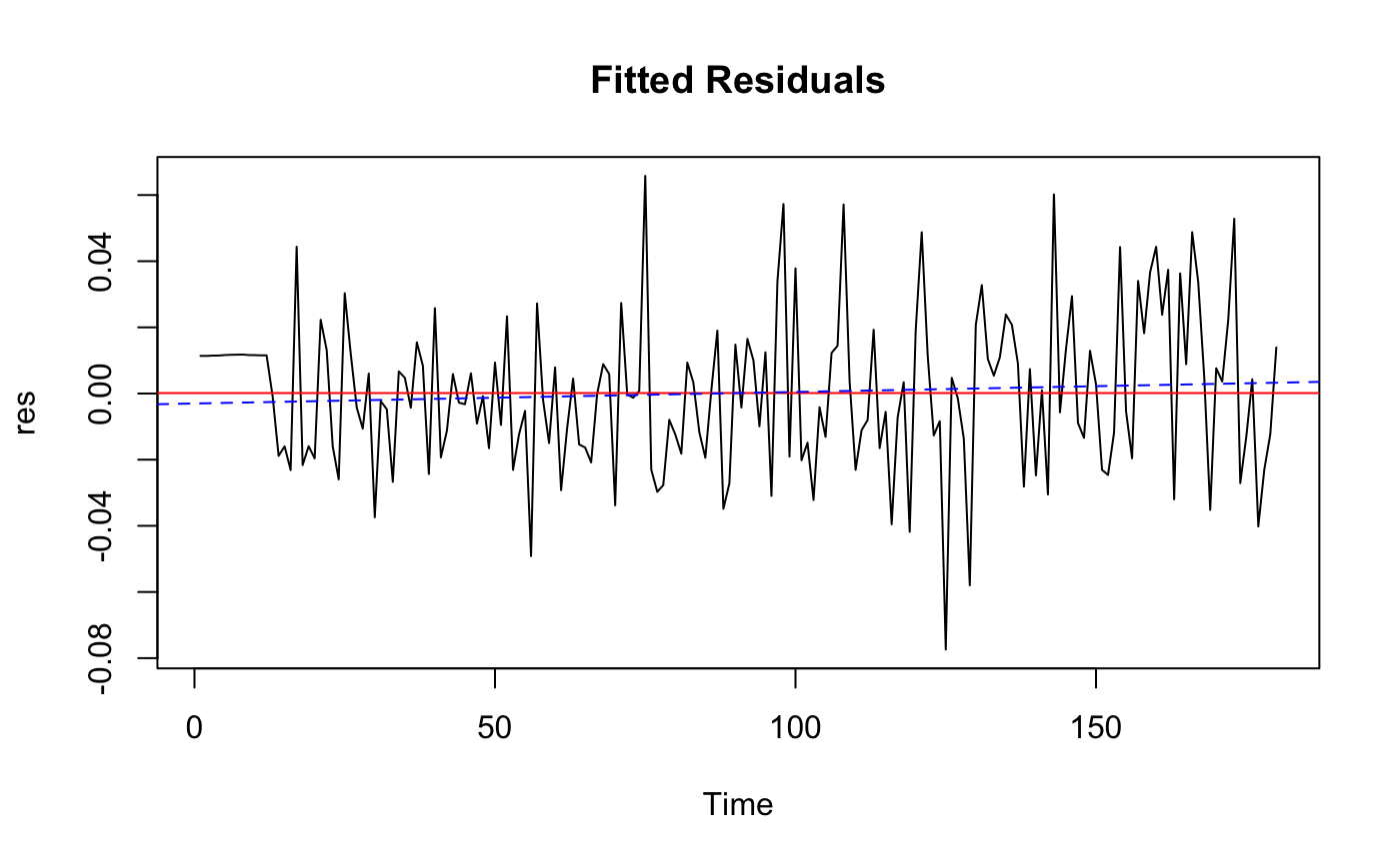
The residual is Roughly WN

  
# Plot diagnostics of residuals
par(oma=c(0,0,2,0))
par(mfrow=c(2,2))
acf(res,main = "res")
pacf(res,main = "res")
# Histogram
hist(res,main = "Histogram",freq = F,density = 40,col = "aquamarine3")
m_res <- mean(res)
std_res <- sqrt(var(res)) 
curve(dnorm(x,m_res,std_res), add=TRUE,col="indianred1")
# q-q plot
qqnorm(res)
qqline(res,col ="blue")
# Add overall title
title("Diagnostics Check for Fitted Residuals", outer=TRUE)

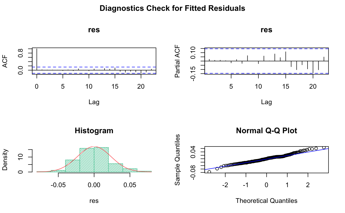
From Histogram and QQ plot we can see the residual is roughly normally distributed.

5.2 Various Box Test

since there are 6 effective coefficient so we take fitdf = 6

  
Box.test(res, lag = 13, type = "Box-Pierce", fitdf = 12) #sqrt(180) is roughly 13
Box.test(res, lag = 13, type = "Ljung-Box", fitdf = 12)
Box.test((res)^2, lag = 12, type = "Ljung-Box", fitdf = 0)#McLeod-Li

	Box-Pierce test

data:  res
X-squared = 3.0571, df = 1, p-value = 0.08039

	Box-Ljung test

data:  res
X-squared = 3.2782, df = 1, p-value = 0.0702

	Box-Ljung test

data:  (res)^2
X-squared = 8.8323, df = 12, p-value = 0.7172

Because the observation of training set is 180, its square root is about 13, so I set lag = 13 in the box tests. Based on three test p-values(>0.05), we can conclude that we fail to reject the null hypothesis thus the Residual is uncorrelated of each other.

6.0 Spectral Analysis

6.1 Periodogram & Kolmogorov-Smirnov Test

  
par(mfrow=c(1,2))
TSA::periodogram(res,plot = T)
cpgram(res,main="Kolmogorov-Smirnov Test")

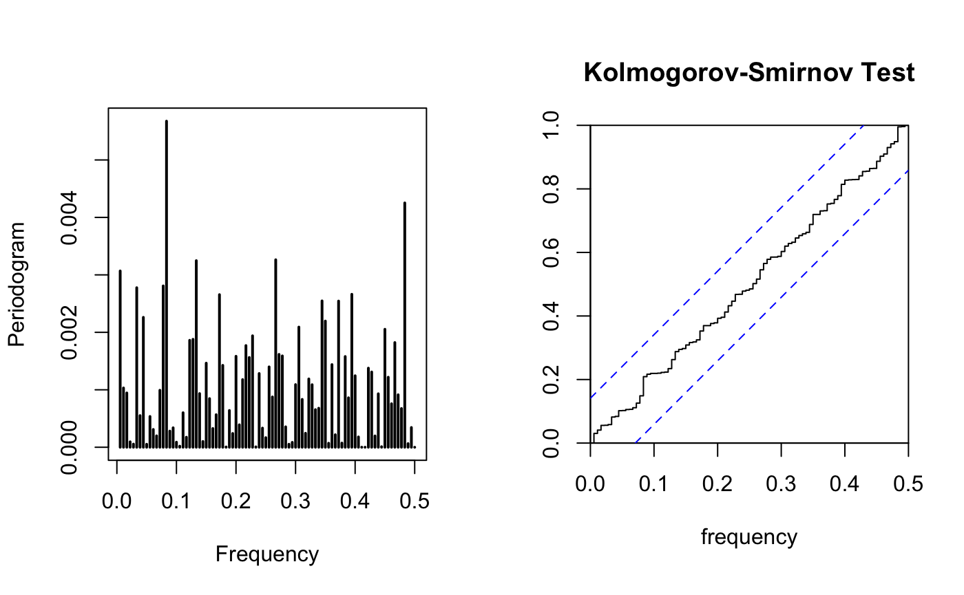
all residual fall between the CI, the residual is Gaussian WN. From the periodogram, I don’t see a dominated frequency

6.2 Fisher test

  
suppressMessages(library(GeneCycle))
fisher.g.test(res)

[1] 0.3939237

since the p-value is larger than 0.05 ,original data is Gaussian distributed(Do not reject $H_0$)

7.0 Forecasting

7.1 set Confidence interval

  
SARIMA <- arima(train.log, order=c(3,0,3), method="ML",
      seasonal = list(order = c(4,1,2), period = 12))
pred.demand <- predict(SARIMA, n.ahead = 12) 
Upperbound <-  pred.demand$pred + 1.96*pred.demand$se 
Lowerbound <-  pred.demand$pred - 1.96*pred.demand$se

7.2 Forecast for training data

  
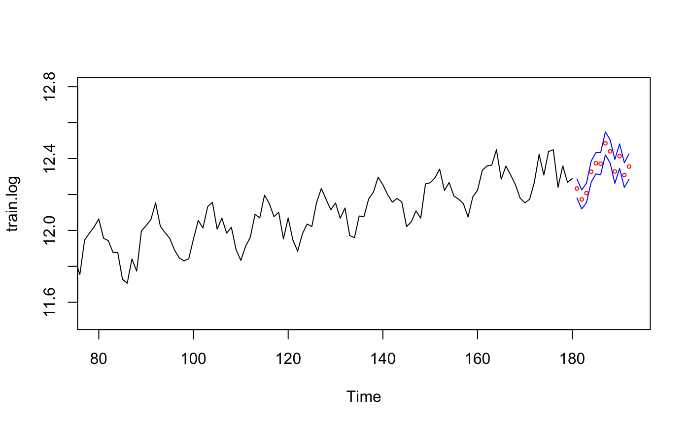
ts.plot(train.log, xlim=c(80,length(train.log)+12), ylim = c(11.5,12.8)) 
lines(Upperbound, col="blue")
lines(Lowerbound, col="blue")
points((length(train.log)+1):(length(train.log)+12), 
       pred.demand$pred, col="red",cex=0.5) # Predicted Value

7.3 Forecasted v.s true value

  
pred.orig <- exp(pred.demand$pred) # transform back
U <-  exp(Upperbound)
L <-  exp(Lowerbound)
ts.plot(train, xlim = c(150,length(train)+12), ylim = c(min(train),max(U)), col="black")
lines(U, col="grey", lty="dashed")
lines(L, col="grey", lty="dashed")
points((length(train)+1):(length(train)+12), pred.orig, col="red", cex=0.5) # Forecasted Value
points((length(train)+1):(length(train)+12), test, col="blue", cex=0.5) # True Value
# legend("bottomleft",pch = 1,col = c("red","blue"))
PerformanceAnalytics::legend("bottomright", pch=1, col = c("red", "blue"), 
       legend = c("Forecasted","True"))

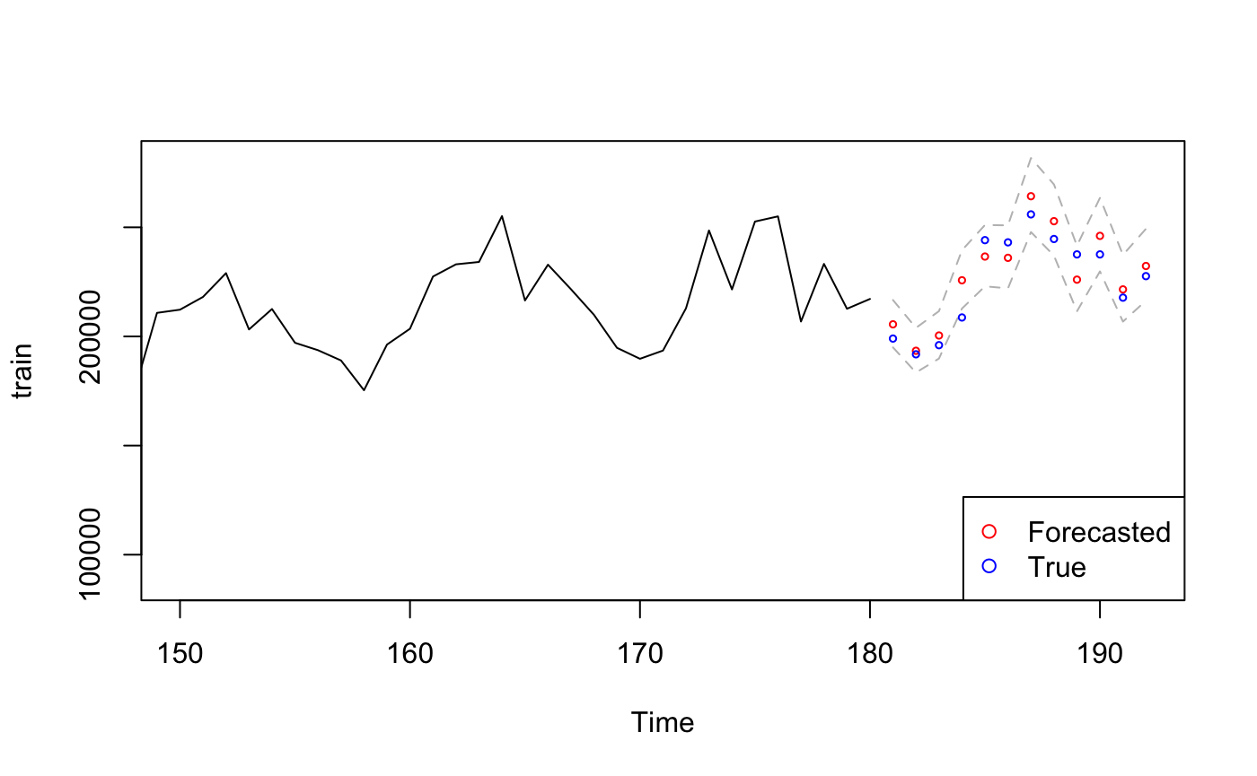
The true value falls in 95% CI of the SARIMA model which indicating the prediction is accurate, the first predicted value even overlaps with the true value which suggesting our model is very good.

8.0 Conclusion

The purpose of this project is predicting future gas demand based on known data sequence, Throughout the process of transforming, differencing, model selection, diagnostic checking, and spectral analysis, the final model I picked is $ SARIMA(3,0,3) \times (4,1,2)_{12} $

Reference

Lecture slides & notes

https://stat.ethz.ch/R-manual/R-devel/library/stats/html/box.test.html

https://cran.r-project.org/web/packages/forecast/forecast.pdf

https://cran.r-project.org/web/packages/TSA/TSA.pdf

https://stat.ethz.ch/R-manual/R-devel/library/stats/html/arima.html

https://github.com/nickpoison/astsa/blob/master/fun_with_astsa/fun_with_astsa.md#arima-simulation

https://cran.r-project.org/web/packages/astsa/astsa.pdf

Time Series Project